Injection Files

Lets look at the different ways we can use injection files in GlitchPop.

Writing a Random Injection File w/ Glitches

To generate a random injection file and the accompanying time series, we can do the following. Lets generate an example with only glitches to save some computing time.

import GlitchPop as gp
import GlitchPop.write

#Generating time series and injection file
#file = True gives us the name of the .json file
ts, filename = gp.write.random_glitch('L1', 'O2', duration = 350, gps = 11e8, mu = 0.25, file = True)

#Plotting time series
plot = ts.plot()

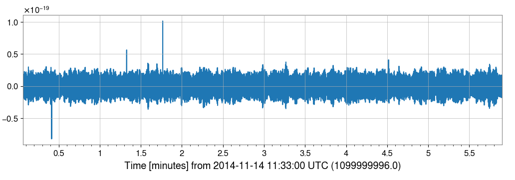
This time series is the object that is create upon writing injection files. There is some rather loud glitches (presumably koi fish) in this time series!

Reading an Injection File w/ Glitches

Continuing on from the last example, lets now read that same injection file and ensure it produces the same time series.

import GlitchPop.read
import matplotlib.pyplot as plt

#Reading injection file
td = gp.read.single_ifo(filename)

#Plotting time series
plot = td.plot()
plt.show()

#Plotting Residuals
plt.title('Residuals')
plt.plot(td-ts)
plt.show()

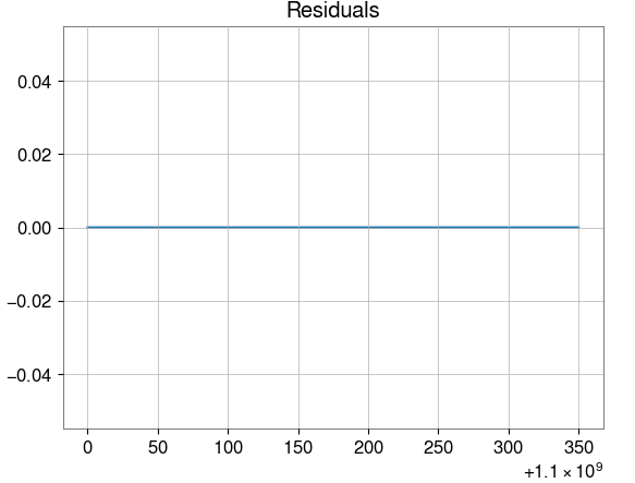
As expected, the residuals between the two time series are a horizontal line at zero. Since this used random (unseeded) generation, users will obtain different plots to this example each time the first code block is ran.

Example Injection File

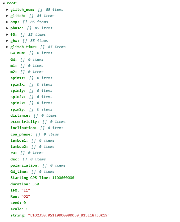
In GlitchPop, injection files are in the form of .json files containing 7 glitch related fields, 20 GW related fields, 6 noise fields and a descriptive string that is used as the file name. The descriptive string (and file name) follows the following format:

IFO abberviation - observing run - duration in seconds - ‘S’ - starting GPS time - ‘_’ - ‘B’ - number of blips - ‘L’ - number of low frequency blips - ‘T’ - number of tomtes - ‘K’ - number of koi fish

The injection file produced from the previous example is shown below (as seen in JupyerLab). Note, although there is many fields, a lot of this fields remain empty, such as x and y spins, depending on the type of simulation one is running.