Multi Detector Simulations

Lets look at the different ways we can generate time series across a 3-detector network using GlitchPop.

‘Deterministic’ Generation w/ Only GWs

To generate a ‘deterministic’ tri-detector simulation (GW can be regenerated running the same commands), we can do the following. The code will produce three time series: one for each of the IFOs. Lets simulate a BNS merger as seen across the network.

import GlitchPop as gp
import GlitchPop.simulate
import matplotlib.pyplot as plt

#Initial time series
h1 = gp.simulate.random_glitch('H1', 'O3a', duration = 100, gps = 13e8, mu = 0)
l1 = gp.simulate.random_glitch('L1', 'O3a', duration = 100, gps = 13e8, mu = 0)
v1 = gp.simulate.random_glitch('V1', 'O3a', duration = 100, gps = 13e8, mu = 0)

#Generating the time series based off O3a
h1, l1, v1 = gp.simulate.determ_tri_ifo_determ(h1, l1, v1, [13e8+87], ['BNS'], [3])

#Plotting spectrograms of BNS signal
qspecgram = h1.q_transform(frange = (10,1024), outseg = (1300000087-10,1300000087+2))
plot = qspecgram.plot()
ax = plot.gca()
ax.set_xscale('seconds')
ax.set_yscale('log', base = 2)
ax.set_ylim(10, 500)
ax.set_ylabel('Frequency [Hz]')
ax.grid(False)
ax.set_title('H1')
ax.colorbar(cmap='viridis', label='Normalized energy', vmin = 0, vmax = 25)

qspecgram = l1.q_transform(frange = (10,1024), outseg = (1300000087-10,1300000087+2))
plot = qspecgram.plot()
ax = plot.gca()
ax.set_xscale('seconds')
ax.set_yscale('log', base = 2)
ax.set_ylim(10, 500)
ax.set_ylabel('Frequency [Hz]')
ax.grid(False)
ax.set_title('L1')
ax.colorbar(cmap='viridis', label='Normalized energy', vmin = 0, vmax = 25)

qspecgram = v1.q_transform(frange = (10,1024), outseg = (1300000087-10,1300000087+2))
plot = qspecgram.plot()
ax = plot.gca()
ax.set_xscale('seconds')
ax.set_yscale('log', base = 2)
ax.set_ylim(10, 500)
ax.set_ylabel('Frequency [Hz]')
ax.grid(False)
ax.set_title('V1')
ax.colorbar(cmap='viridis', label='Normalized energy', vmin = 0, vmax = 25)

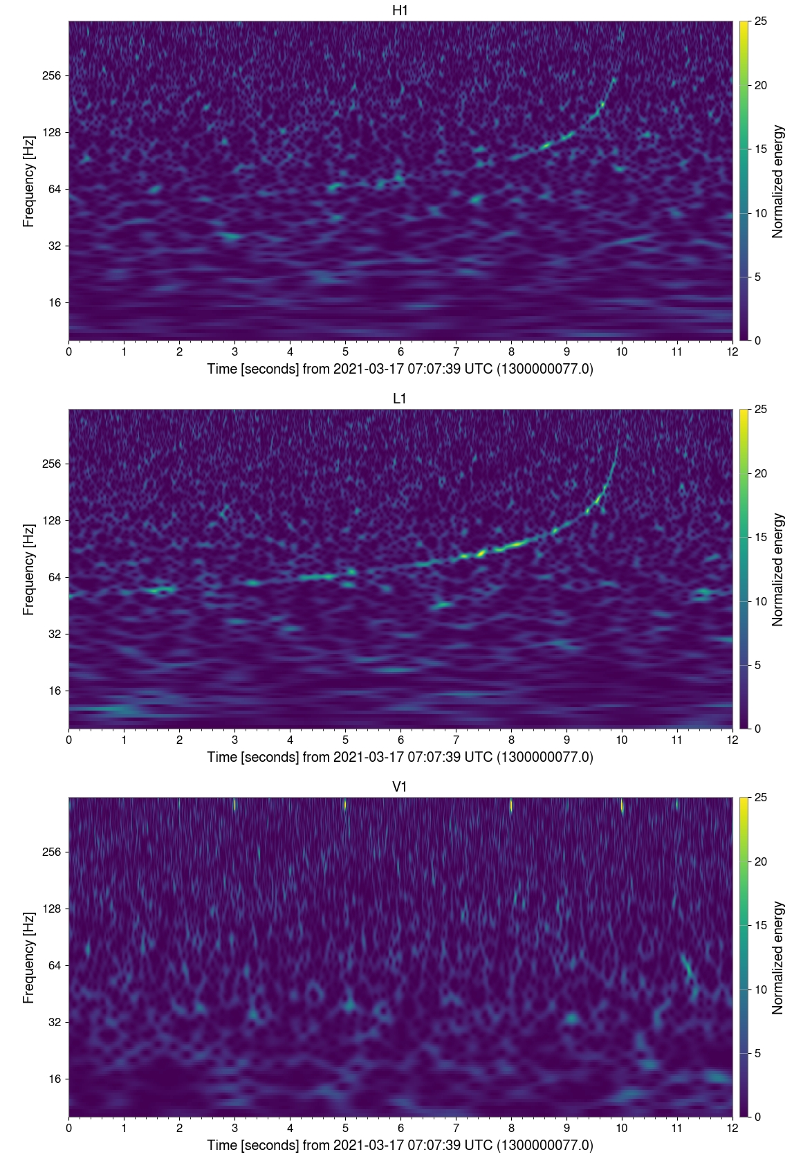
As expected, the signal is most visible in Livingston (L1). Note, this is actually ‘quasi-deterministic’ as the initial time series (ie. the Gaussian nosie) are not generated with a random method. As a result, one will obtain slightly different spectrograms upon running this.

Deterministic Generation w/ GW & Glitch

Now demonstrating GlitchPop’s ability to generate GWs and glitches simultaneously. Lets generate a signal similar to GW170817 (arXiv:1710.05832) where there is an overlapping GW and glitch.

import GlitchPop as gp
import GlitchPop.simulate
import matplotlib.pyplot as plt

#Initial time series
#H1 and V1 are glitch free but require empty brackets and at least one seed (for noise)
h1 = gp.simulate.determ_glitch('H1', 'O3a',[], [], [10], duration = 100, gps = 13e8)
l1 = gp.simulate.determ_glitch('L1', 'O3a', ['blip'], [13e8+85], [10], duration = 100, gps = 13e8)
v1 = gp.simulate.determ_glitch('V1', 'O3a', [], [], [10], duration = 100, gps = 13e8)

#Generating the time series based off of O3a
h1, l1, v1 = gp.simulate.determ_tri_ifo(h1, l1, v1, [13e8+87], ['BNS'], [3])

#Plotting whitened time series
hw, lw, vw = h1.whiten(), l1.whiten(), v1.whiten()
plt.plot(hw.times, hw.value, color = 'red', label = 'H1')
plt.plot(lw.times, lw.value,label = 'L1')
plt.plot(vw.times, vw.value,color = 'purple', label = 'V1')
plt.xlim(13e8+84,13e8+87.5)
plt.ylim(-5,5)
plt.axvline(x = 13e8+87, label = 'Merger', linestyle = '--', color = 'orange')
plt.legend()
plt.show()

#Plotting spectrograms of BNS signal
qspecgram = h1.q_transform(frange = (10,1024), outseg = (1300000087-5,1300000087+1))
plot = qspecgram.plot()
ax = plot.gca()
ax.set_xscale('seconds')
ax.set_yscale('log', base = 2)
ax.set_ylim(10, 500)
ax.set_ylabel('Frequency [Hz]')
ax.grid(False)
ax.set_title('H1')
ax.colorbar(cmap='viridis', label='Normalized energy', vmin = 0, vmax = 25)

qspecgram = l1.q_transform(frange = (10,1024), outseg = (1300000087-5,1300000087+1))
plot = qspecgram.plot()
ax = plot.gca()
ax.set_xscale('seconds')
ax.set_yscale('log', base = 2)
ax.set_ylim(10, 500)
ax.set_ylabel('Frequency [Hz]')
ax.grid(False)
ax.set_title('L1')
ax.colorbar(cmap='viridis', label='Normalized energy', vmin = 0, vmax = 25)

qspecgram = v1.q_transform(frange = (10,1024), outseg = (1300000087-5,1300000087+1))
plot = qspecgram.plot()
ax = plot.gca()
ax.set_xscale('seconds')
ax.set_yscale('log', base = 2)
ax.set_ylim(10, 500)
ax.set_ylabel('Frequency [Hz]')
ax.grid(False)
ax.set_title('V1')
ax.colorbar(cmap='viridis', label='Normalized energy', vmin = 0, vmax = 25)

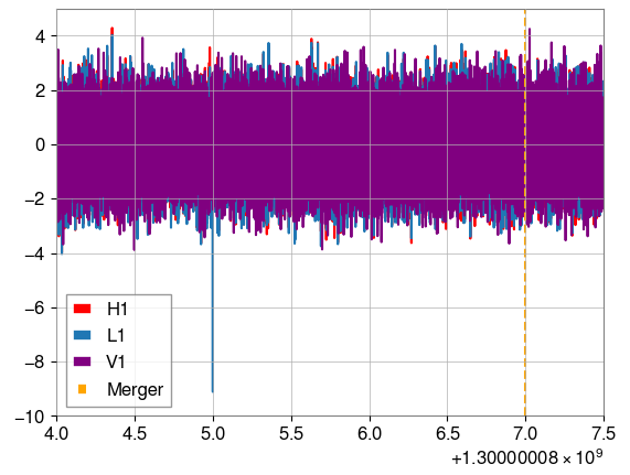
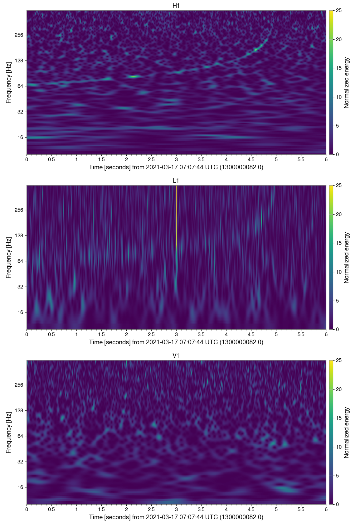
BNS merger across H1, L1 and V1 w/ overlapping blip at L1

From this, we can see how a blip glitch interferes with an overlapping GW signal. In the first example, the chirp was most visible in L1 but after the glitch, the signal is weaker. The blip is also noticable in the whitened strain around the 5.0 mark.

Note, the code for generating this is very similar to the first example. However, this uses a complete deterministic (seeded) method and injects a GW.