Single Detector Simulations

Lets look at the different ways we can generate single detector time series using GlitchPop.

Deterministic Generation w/ Only Glitches

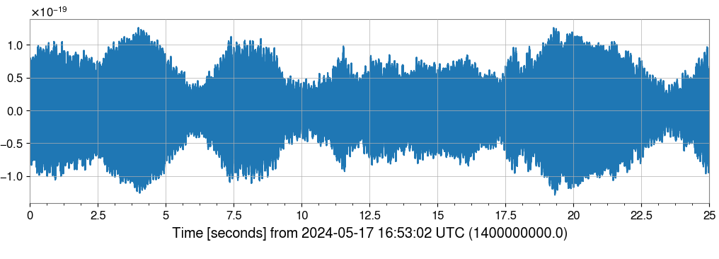
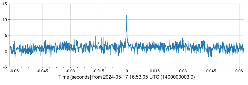
To generate a fully deterministic time series (can be regenerated running the same commands), we can do the following. Note, we can choose the type, the random seed and the location of each generated glitch.

import GlitchPop as gp
import GlitchPop.simulate
import matplotlib.pyplot as plt

#Generating a time series based off of L1 during O3b
ts = gp.simulate.determ_glitch('L1', 'O3b', ['blip', 'tomte', 'lfb', 'koi'], [14e8+3, 14e8+4, 14e8+5, 14e8+6], [1,2,3,4], duration = 25, gps = 14e8)

#Plotting full time series
plot = ts.plot()

#Whitening and zooming in on blip
tsw = ts.whiten()
tsw.plot()
plt.xlim(14e8+3-1/16, 14e8+3+1/16)
plt.ylim(-5,15)

Random Generation w/ Glitches and GWs

To generate a random time series (cannot be regenerated running the same commands), we can do the following. Although usually not explicitly seen in the coloured strain, this time series will contain both gravitational wave signal(s) and glitches.

import GlitchPop as gp
import GlitchPop.simulate

#Generating a time series based off of H1 during O3a
ts = gp.simulate.random_gw('H1', 'O3a', gps = 12e8, duration = 500, mu_glitch = 0.05, mu_gw = 0.005, probs_gw = [1,0,0], probs_glitch = [1,0,0,0])

#Plotting full time series
plot = ts.plot()

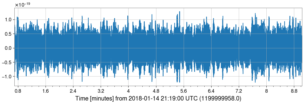
Notice here, we set the probabilities of the GWs and glitches so that only BHBH signals and blips were generated. The ‘mu’ arguments are the Poissonian rate or glitches/GWs expected per second. For this example, we expect 25 blips and 2.5 BHBH signals.